On the use of instability indicators in exploring inter-decadal GDP variability

Introduction

The following text aims to contribute to the literature on the inter-decadal dynamics of the macro-economy, using a novel analysis of historical GDP data. The study is motivated by an interest in the limits to economic growth (Meadows et al 1972; Jackson and Webster 2016, Jackson 2017, Victor 2008), whether these arise from resource availability (Meadows et al 1972), environmental constraints such as climate change (Solomon et al 2007; Raworth et al 2012) or secular inter-decadal dynamics (Summers 2013; Gordon 2016). In particular, we are interested in the temporal variability of recession cycle properties, and their utility as indicators of GDP ‘instability’.         

Recession cycles, i.e. de-trended GDP variability or oscillations, have been a fundamental subject of economic research and debate for around two centuries. Within this debate, there are four widely discussed timescales of variability. Kitchin (1923) introduces the shortest 3-5 year timescale and argues that it is related to the renewal of business inventories. Juglar (1860) describes a medium 7-11 year timescale and relates it to business capital investments. Kuznets (1930) introduces a longer 15-25 year scale and links it to infrastructure investment. Finally, Kondratieff (1979) describes a 45-60 year scale and relates it to technological change. However, following the initial observations of these scales, there is little consensus on their definition and their driving mechanisms (Hayek, 1933; Keynes, 1936; Goodwin, 1967). Further, there is little discussion on their interaction or inter-decadal variability.

Kuznets and Kondratieff scale variability are of particular interest because of their likely importance to the inter-decadal macro dynamics. Kondratieff-scale variations are commonly referred to as k-waves (or long-waves) and have been associated with a number of forcing mechanisms, from political upheaval to resource availability (Grinin et al 2012). Interestingly, Kuznets scale variability is additionally associated with inter-decadal (secular) trends in inequality, and with the Kuznets-curve, which implies a relation between GDP per capita and inequality (Milanovic 2016).

Over recent decades, the growth rates of many advanced economies, particularly USA, UK, Japan, Italy, France, and Germany (which dominate the G7 group), have declined. This decline is referred to as ‘secular stagnation’ in the literature (Summers 2013). The cause of this decline is poorly understood (Summers 2013; Gordon 2012, 2016). It is associated with a number of notable inter-decadal trends, referred to as ‘head-winds’, discussed by Gorden 2012. The time-scale of Secular Stagnation is comparable to the theoretical timescale of Kuznets (1930) variability, or half the timescale of Kondratieff variability. Further, prolonged periods of low growth have previously been discussed in relation to Kondratieff scale variability (e.g. Schumpeter 1939).

Although multiple authors have analysed the relationship between the GDP growth rate and de-trended GDP variability, they have tended to focus on short timescale phenomenon. For example, Ramey and Ramey (1994) and Hnatkovska and Loayza (2005), both provide evidence of a negative correlation between economic growth and its volatility. Reinhart and Reinhart (2015) provide an overview of this subject and new analysis. They find a negative correlation between the magnitude of crises leading to a recession and the growth rate following a recession. Further analysis of long-term GDP variability and secular stagnation is timely considering the severity of the recent recession and the immediacy of long-term policy issues associated with global challenges (IPCC 2007; Meadows et al 1972; Raworth et al. 2014).

The following section reviews the economics literature on instability indicators and the theoretical basis of the indicators used by the complex systems sciences. Section 3 sets out the methodology of the study, and in particular reviews the two indicators that are used to quantifying the temporal variability of GDP ‘stability’. Section 4 documents the results of applying these instability indicators to a range of GDP time series. Section 5 provides some synthesis of the previous sections, additional qualitative analysis and links to the wider literature. Section 6 provides a summary and concludes the paper.

2 Instability indicators and the theory of critical slowing down

The following section outlines the current economics literature on instability indicators. Following Reinhart and Reinhart (2015), a high-quality indicator of instability could provide invaluable insights. However, despite instability indicators being an active topic of research, there is little consensus on their utility.

Indicators of financial viability (e.g. Altman’s Z-score) at the micro level (Shumway 2001; Chava and Jarrow 2000) have been aggregated to produce Macro-scale indicators (e.g. Bharath and Shumway 2004). However, these indicators are imperfect, as they do not account for firm-firm and firm-institution dynamics (Eijfinger 2011).

Novel data analyses techniques, borrowed from the complex systems sciences, have been used to explore economic instability. For example, Ramirez and Rodriguez (2011) have analysed the Dow Jones Index (DJI) in terms of the variability of its ‘entropy’, where they observe a 22-year cycle in the DJI data. Quax et al. (2013) have analysed variability in the ‘information dissipation length’ of interest rate swaps (IRS), finding early warning signals in the period leading to the Lehman Brothers collapse. Tan and Cheong (2014) have analysed the dynamics of instability in the U.S. housing market. Furthermore, Diks Hommes and Wang (2015) use the time-variability of variance and autocorrelation (auto-regression) to quantitatively the instability of financial indices. These novel techniques provide useful new insights. However, they tend to deal with relatively short time-scales and mainly with financial indicators.

The instability indicators used by Diks Hommes and Wang (2015) are of particular interest to this paper. They are derived from the fundamental work of Wiessenfeld (1985) and Wissel (1984), who argue that both the time required for an oscillating system to adjust to perturbations and the amplitude of its oscillations increase as a system’s restoring forces weaken. This slowing down and amplification of a system’s oscillations is referred to as ‘Critical Slowing Down’ (CSD). Typically CSD is associated with ‘critical transitions’ or ‘tipping points’ (e.g. Lenton 2011). However, Kefi et al. (2013) expanded the theory of CSD to include general situations of decreasing stability in the face of weakening restoring forces. These restoring forces can also be thought of as negative feedback (or balancing) loops. As the negative feedback loops weaken, the potential for instability increases.

CSD theory is very general; it can be applied to any time-periodic system that is comprised of deterministic and stochastic components. A number of authors have developed instability indicators to identify CSD behaviour (e.g. Kleinen Held and Petschel-Held, 2003; Dakos, 2008;). This approach is inspired by complexity economics. Where, a growing body of literature describes economic systems in terms of complex systems, influenced by multiple equilibria, similar to ecology or climate systems (e.g. Dakos et al. 2008; Dakos et al. 2012; Sornette, 2009; Scheffer et al., 2009; Quax et al., 2013).

The qualitative behaviour of CSD described by Wiessenfeld (1985) and Wisel (1984) is best illustrated with an abstract example. Consider an object that is suspended between two springs, in a windy environment (the spring-object-spring system; Figure 1a). The springs provide a deterministic restoring force (black arrows), and the wind provides a series of stochastic perturbations that force the object to oscillate. If the springs are strong (strong restoring), oscillations are fast and small. If the springs are weak (weak restoring), oscillations are slow and large. If the relative strength of the springs becomes weaker over time, then the oscillations of the system transition from small and fast to large and slow (Figure 1b). This transition is characteristic of CSD behaviour. An additional example is given in Appendix I.

A premise of our own study is that CSD theory may also be applicable to economic systems. In the case of a national economy, for example, restoring forces might include the relationship between profits and wages, the relationship between investment and discretionary spending, or the price mechanism for commodities. In the next section, we describe some quantitative methods for identifying CSD.

3 Methods for quantifying observation of CSD

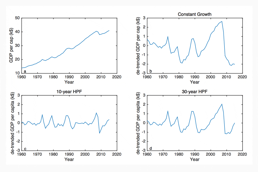
Multiple approaches have been suggested for identifying CSD behaviour in time-series data. The following subsections outline the two leading methods. Additional complimentary methods are discussed in Appendix II. The recent UK per capita GDP time series is used as an example dataset (Figure 3a).

3.1 De-trending

CSD behaviour is identified by analysing the oscillations of a system. However, GDP datasets typically have large non-linear growth trends that can obscure these oscillations from analysis. As with similar analyses in other fields (Lenton 2011), the long-term trend must first be removed from the time series, so that short term variations become identifiable. The choice of de-trending method is critical to CSD analyses. For illustration, here the trend is first removed with the assumption of a constant growth rate (Figure 3b). The resulting series is then ‘smoothed’ by using two forms of the Hodrick-Prescott filter (HPF), which allow the growth rate to vary over the time series. The time window over which the growth rate is averaged by the HPF filter, is typically chosen as ~7-11 years. However, this standard choice is biased by the assumption that GDP variability is dominated by oscillations with that period (the business cycle; Lee 1955). Figure 3c shows the HPF de-trended time series with a standard, ~10-year average growth rate (Lee 1955). Figure 3d, shows the HPF de-trended time series with a ~30-year averaged growth rate.

Inspection of Figures 3a, 3b and 3d suggests that the period and magnitude of the recession cycles have increased between 1960 and 2010, indicative of a period of CSD. However, this behaviour is not apparent in Figure 3c. To test this further, in the following text, the validity of results is examined using a range of de-trended averaging periods (ranging 5-40 years), for all analyses. For example, for Figure 3, the trend in CSD instability is found to be significant for all de-trending methods shown (3b-d).

3.2 Instability indicators: autocorrelation

A widely used indicator of CSD is the AR1 autocorrelation (Held and Kleinen 2004; Lenton 2011). AR1 is an estimate of the correlation between a given time series (e.g. per capita GDP) and a one period lag of the same time series. When applied to GDP time series, AR1 provides a measure of the typical time-scale of the variability, or oscillations, of an economy. So, for example, a rapidly oscillating economy expresses a low AR1 value and a slowly oscillating economy expresses a high AR1 value. Furthermore, a relatively low (high) AR1 value implies that the restoring forces of the economy are relatively strong (weak).

In order to provide an estimate of the change in AR1 with time, the local AR1 is estimated in a moving window of data points. Where the size of the calculation window can have a large effect on the resulting magnitude of AR1. Lenton et al. (2011) argue that the most appropriate window size is typically half the length of the time series. In this study, the AR1 indicator is estimated with window sizes ranging from 5 to 40 years and then inter-compared to test for the robustness of estimates.

A positive (increasing) trend in AR1 indicates that the oscillations of the system are changing from small and fast to large and slow. In other words, the typical time-period of variability of the system is getting longer and the strength of the system’s restoring forces is diminishing. CSD theory suggests that a tipping point is most likely to occur as the autocorrelation function approaches 1 (Lenton 2011). At this point, the oscillations of the system are exceptionally large and slow and the system may change rapidly into a new state. However, the magnitude of AR1 is strongly affected by the method of de-trending and choice of calculation window. It is therefore widely suggested that the trend in AR1 is more insightful than its absolute magnitude (e.g. Lenton 2011).

Figure 4 shows the AR1 autocorrelation, for the UK GDP time series, calculated using 30-year HPF de-trended GDP, and a 25-year moving window in AR1. AR1 is shown to increase by around 30% between the 1975 and 2005. This implies that over this period, the de-trended oscillations of the UK GDP per capita have slowed down and that the restoring forces maintaining the equilibrium growth path have diminished over this time.

The significance of the trend in AR1 (i.e. a linear fit to Figure 4) can first be tested using a Kendall Rank correlation test or a Pearson correlation test. For both these tests, the trend in Figure 4 was found to be significant (p<0.05). A more robust significance test is achieved using a Monte-Carlo method, where the observed trend is compared to a thousand random re-arrangements of the same time series. In this test, if the strength of the trend in AR1 is found to be within the top 5% of the random rearrangements, it said to be significant. For this test, the trend in Figure 4 was also found to be significant (p<0.05).

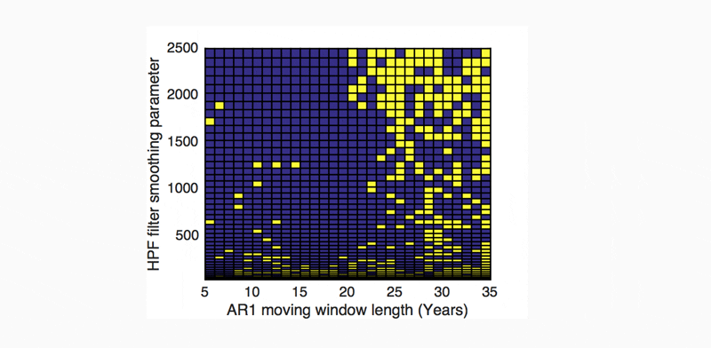
Finally, it is reiterated that the calculation parameters used in estimating AR1 can have a large impact on the resultant trend in AR1. The significance of a trend in AR1 (e.g. Figure 4) was tested using both Kendall Rank and Monte-Carlo tests, for a large range of (de-trending, HPF filter) smoothing parameter values and ‘moving window’ sizes. If the trend is found to be significant for the majority of calculation parameter values, then it is considered to be sufficiently significant for this analysis. Figure 5 shows this distribution for Figure 4 and reveals that the recent (1960-2015) trend in the UK’s GDP-AR1 (Figure 4) was significant for the large majority of reasonable parameter values.

3.3 Instability indicators: variance

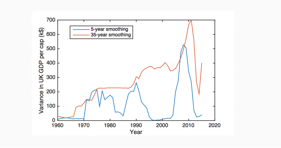
A further indicator of instability is the variance. Indeed, the variance of de-trended GDP is widely used as an indicator of CSD (increasing instability; Wiessenfeld 1985; Wisel 1984). The variance is estimated using the same de-trending method and moving window as the AR1 indicator, described in the previous section.

The trend in variance is, unfortunately, likely to be biased by the size of an economy. It is intuitive that the magnitude of the oscillations of an economy is equated to the size of the economy. Then its de-trended oscillations are expected to increase in absolute magnitude as an economy grows. Therefore, one expects a growing economy to additionally exhibit a spurious positive trend in the variance of its de-trended GDP. The simplest correction for this is to express the variance as a percentage of the GDP. However, further research is required to optimise this correction. Unless stated otherwise, no correction to the variance is made in this text and therefore the AR1 indicator is qualitatively preferred over the variance in our discussion (Section 4).

The variance indicator was tested for significance using the same method as for AR1, i.e., using the Kendal Rank correlation and Monte-Carlo tests over a wide range of estimation parameters. The value of the variance for the UK GDP time series is shown in Figure 6. This trend is consistently significant (p<0.05) for smoothing parameter values of 10-40 years and ‘moving window’ sizes of 5-30 years.

4 Analysis: application of CSD (instability) indicators to global GDP datasets

The AR1 and variance indicators were used to explore the Madison Project dataset of yearly per capita GDP. Data are available for 9 countries between 1820 and 2010, for 20 countries, between 1900 and 2010, and for around 80 countries between 1930 and 2010 (The Maddison-Project 2013).

The extended dataset, between 1820 and 2010, is available for USA, UK, Denmark, France, Italy, Holland, Sweden, Australia and Indonesia. These invaluable data show fascinating variability in the AR1 and variance indicators for almost two centuries. They highlight periods of high and low AR1, with typical time scales of 20-60 years, supportive of Kondratieff and Kuznets theory. No clear internationally dominant pattern is apparent pre-1900. However, the early data for the UK show a (highly significant) general positive trend in AR1 between 1820 and 1950 (Figure 7).

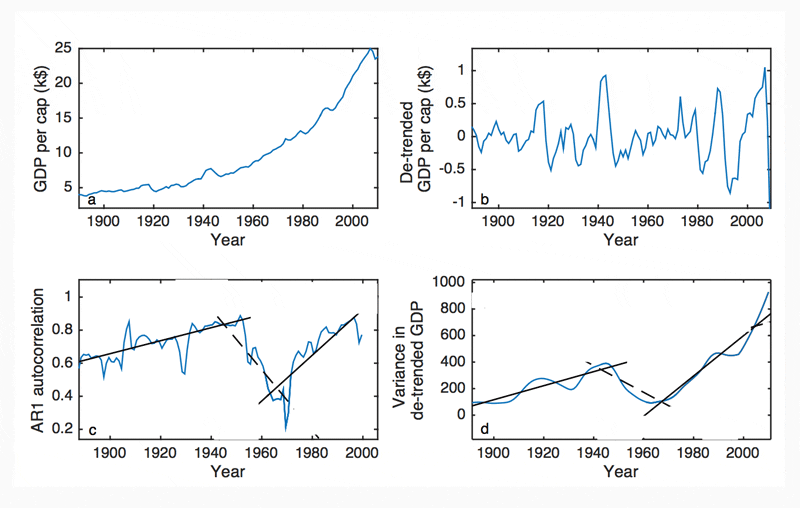
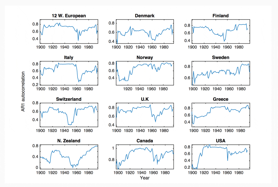
Following 1900, a dominant pattern in AR1 and variance between 1900 and 2010 is evident. This pattern is best described as an increasing trend leading up to a period of high instability between 1915-1950, a decline from 1940 leading to a period of high growth around 1960-1970, followed by a second increase from 1950 to present day (Figure 8). The period of high instability between 1915 and 1950 notably encompasses the First World War, The Great Depression and the Second World War.

This dominant pattern is observed in 70% of high GDP countries and 5% of low GDP countries. It can be defined by three linear fits, as shown in Figure 8c-d. These fits are significant for around half of high GDP time series. Notable countries that fit this pattern significantly include, the U.K, USA, Canada, France, Germany, Denmark, Italy, Holland, Sweden (Figure 9). At least two components of this fit are significant for 75% of high GDP countries.

The AR1 and variance indicators were additionally used to explore the recent yearly GDP per capita data, between 1960 and 2015, for around 130 countries, provided by the World Bank (World Bank 2016). A significant trend (p<0.05) in AR1 is found in approximately 60% of countries. 40% show an increasing trend, 20% show a decreasing trend. The increasing AR1 group contains many large western economies such as, the United States, Canada, Australia, the United Kingdom, and Italy. It also contains large eastern economies, such as China, Indonesia and India (Appendix III).

Finally, the AR1 and variance indicators are used to explore the recent quarterly per capita GDP data, between 1960 and 2015, for 20 countries (mainly high GDP nations), provided by the OECD (OECD 2016). A significant trend (p<0.05) in AR1 was found in approximately 90% of countries. 70% showed an increasing trend, 20% showed a decreasing trend. The higher resolution data provides greater detail, and higher significance for recent trends (Appendix IV).

5 Discussion

5.1 On the CSD framework

The findings of this study suggest that CSD instability indicators may be a potentially invaluable tool in exploring inter-decadal macro dynamics. For example, the behaviour of the spring-object-spring system described in the introductory section is qualitatively similar to the behaviour of many non-equilibrium growth models. These include the Goodwin cycle (1967), Minsky’s financial instability hypothesis (1992) and the Minksy-models researched by Keen (2013) and others. In a general regard, CSD instability indicators have been shown to be useful for several other fields of academic research (e.g. Lenton 2011; Dakos et al. 2008; Kefi et al. 2013).

However, it is important to clarify what exactly is meant by ‘instability’ in the context of analysing GDP time series with the AR1 and variance indicators. Specifically, it does not refer to variability in the GDP per se. Rather, a state of instability refers to a state of relatively slow, large, recession cycles. It can be thought of as a state of weak restoration to the equilibrium growth path or a period where an economy takes a relatively long time to return to its equilibrium growth trend, following a perturbation. CSD theory suggests that a movement from a stable to an unstable state implies the onset of a ‘critical transition’ or tipping point (e.g. Lenton 2011). However, a clear tipping point, following a period of CSD, is not apparent in any of the GDP time series examined in this study. Following Kefi et al. (2013), instability indicators may be viewed as indicators for changes in the behaviour, interactions, inputs, or structure, of an economy.

Here, the term ‘instability’ spuriously implies an undesirable system state, i.e. counter to a notion of prosperity. However, it is unclear whether periods of ‘stability’ or ‘instability’ (in this context) are optimal for the wellbeing or prosperity of a society. For example, there are multiple inter-decadal trends and significant events which which have occurred in the same time period as the observed trends in AR1 (Gorden 2012). These include the decline in the quality of energy resources (Murphy and Hall 2011), national/international conflicts, political changes, demographic shifts (Jiang 2011), trends in labour productivity (Baumol 1966, Jackson 2017) and clusters of technological innovation (Schumpeter 1939). There are therefore many opportunities for long-term trends to reinforce each other and thus to facilitate unintuitive outcomes, such as prolonged recessions that reduce inequality (Milanovic 2016) or international conflicts. They may also provoke spurious correlations. Furthermore, it is noted that in a high GDP nation, GDP is a poor indicator of personal or societal wellbeing (e.g. Jackson 2017; Douthwaite 1992). It is evident therefore, that great care must be taken in the interpretation of the results of analyzing the GDP using CSD instability indicators.

In further research, it would be ideal to use a larger range of CSD indicators and other analyses in unison. Extensive work is required to explore additional instability/CSD indicators and to explore the growth bias in the variance indicator. Moreover, work is required to strengthen the link between CSD theory and the economic literature.

5.2 On the results of our analysis

The most robust result of our analysis is the observation of a dominant pattern in AR1 and variance in historical data. This pattern implies an increase in instability between 1850 and 1950, a decline in instability, between 1940 and 1970, then a second increase from 1960 to 2000. This pattern is most apparent for the large GDP nations, particularly the United States, the United Kingdom, Canada, New Zealand and Ireland. The consistency of this pattern in the AR1 and variance indicators (Figure 8) is highly supportive of its validity, the validity of the indicators and the validity of the general method.

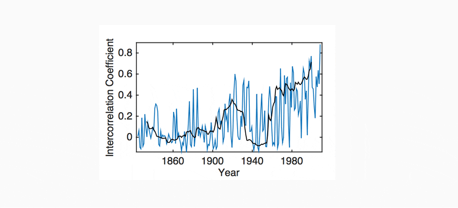
An additional, less understood, indicator of instability can be derived from the inter-correlation of nations in the global economy. It illustrates a similar pattern to that observed in the AR1 and variance indicators, providing additional support for the argument, in the sense that, as a clustered system undergoes CSD, the oscillations of its constituent components become increasingly correlated. This change in behaviour can be quantified for the global economy by estimating the inter-correlation coefficient between multiple GDP time series (Also referred to as intra correlation coefficient; ICC). This coefficient was estimated for the Maddison project historical per capita GDP data, for the 9 countries with the longest available time series (USA, UK, Denmark, France, Italy, Holland, Sweden, Australia and Indonesia; 1820-2010; Figure 10). Here, a similar pattern to that observed in the AR1 and variance indicators (Figure 8) is observed. However, this type of indicator is poorly understood, the significance of its trends is difficult to estimate and it should therefore be interpreted qualitatively.

One particularly interesting question arises from our analysis. Given the evidence of a slowing down in the growth rate in so-called advanced western nations, is there a correlation between a slowing down of the growth rate and a rise in economic or financial instability? Piketty (2014) has argued that a slowing down of the growth rate may lead to rising inequality. Douthwaite (1992) and others have argued that growth is necessary for the stability of a capitalistic economy, particularly (Binswanger 2009) where this entails a debt-based money system. Jackson and Victor (2015) showed that a quasi-stationary economy with debt-based money and a long-term zero trend in the growth rate is formally possible. But Jackson (2009, 2017) has also highlighted potential instabilities that arise when a capitalistic economy slows down.

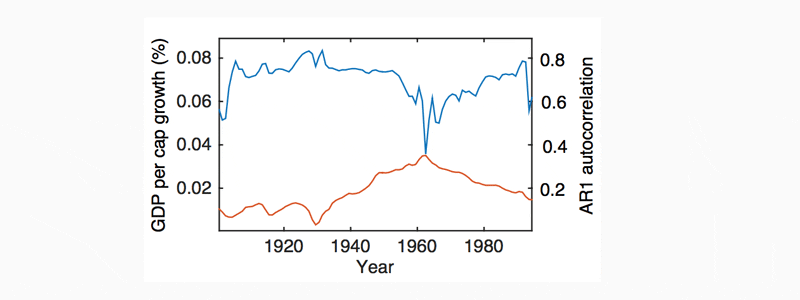
A qualitative analysis carried out in this study suggests (Figure 11) that an inverse relationship (correlation) may exist between the AR1 indicator and the GDP growth rate. However, this relationship is variable and difficult to quantify. This relationship is most apparent in the aggregate per capita GDP datasets, such as the OECD aggregate, the G7 aggregate and the Western Europe aggregate. These aggregate time series express a strong negative (inverse) correlation between AR1 and the GDP growth rate, between 1900 and 2015. However, this relationship is not observed before 1900 and it is only present for 25% of high GDP countries in national historical (1900-2015) data, namely: Denmark, Finland, Italy, Switzerland, and New Zealand. This relationship is most prominent in the recent (1960-2015) national per capita GDP datasets, for around 40% of recent countries and specifically 60% of high GDP national datasets.

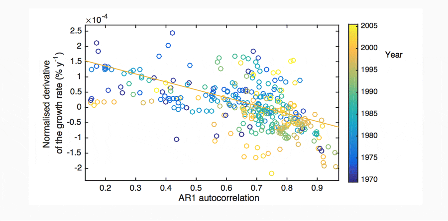
Additional analysis suggests that AR1 may be better correlated with the change in the growth rate (the time derivative of the growth rate) than the growth rate itself, where relatively high AR1 values are associated with decelerating GDP growth. This relationship is found to be significant for around 25% of national datasets. However, it is found to dominate the large GDP nations. It is found to be significant for 8 of the 10 largest economies in the recent data, constituting around 66% of global GDP (in 2015; Figure 12). Germany and France are the two highest GDP countries that only inconsistently follow the relationship.

5.3 On the wider literature

The results of our analysis relate to multiple discussions on long-term macroeconomic dynamics. Notable examples include: the arguments from k-wave theory that highlight a repeating long-term (20-60 year) cycle in GDP growth rate (Grinin, Devezas and Korotayev, 2012); the work of Reinhart and Reinhart (2015) who highlight an inverse relationship between economic crises (GDP volatility) and growth; a study by Harras and Sornette (2008), proposing that market instability develops endogenously by a self-organizing market process, during periods of low growth; and the work of Minsky (1992) and Keen (2010), who argue that instability develops endogenously in financial systems. Finally, our results may relate to the work of Brucker and Gruner (2011), who find a link between declining growth rates and political instability.

6 Conclusions

This paper attempts to contribute to the discussion on the economic consequences of a slowing down in the growth rate. It utilises novel data analysis techniques developed by complex systems science to explore the Critical Slowing Down (CSD) of national economies as indicated by the patterns of instability evident in long-term GDP datasets. In particular, it emphasises inter-decadal (k-wave) scale variability in the growth rate.

We conclude that statistical analyses measuring CSD may provide an invaluable tool for analysing GDP variability, for predicting instability and for understanding the complex dynamics of the national and international macro-economy.

Analysis of historical data has highlighted insightful long-term trends in the ‘stability’ of national economies. A dominant pattern in instability indicators is found in the majority of high GDP nations following 1900. This pattern is characterised by increasing instability from 1900 leading into the 1940s, followed by a decline between the 1930s and the 1970s, then a second increase in instability from the 1960s to 2010.

Considerable further work is required, particularly to diversify the range of instability indicators, to better understand the link between instability and growth, and to better understand the link between instability indicators and economic theory.

Ultimately this work is inspired by an interest in long-term macro dynamics and global challenges, such as climate change. An optimal mitigation strategy for environmental challenges may be a net intentional decline in economic output, associated with a ‘more fun less stuff’ reduced GDP approach (Jackson 2009). Many authors have highlighted that a long run decline in GDP does not necessitate a decline in living standard, particularly for the high GDP per capita nations (Druckman et al. 2008; Reay 2006; Jackson 2009; Sen 1985; Townsend 1979). Regardless, it is likely that the dominant economies will face long-run periods of declining growth or GDP, driven by global challenges, in the coming decades to century (Meadows, Randers and Meadows 1972). Further, a significant proportion of the appropriate climate change mitigation strategies are likely to drive a downward pressure on the GDP growth rates (Stern 2006; Jackson 2009). Our understanding of the national and international dynamics of a declining political-economy is poor. It is clear that intensive research is required to inform long-term policy advice for the global challenges of the coming century (Beddington 2009).